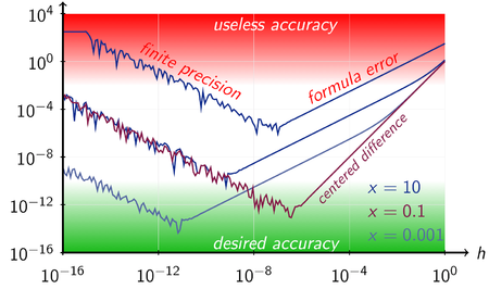
Mastering Derivatives From Math to Code

Learn the mathematical concept, see how it translates into Python code, and discover three numerical differentiation methods - forward, backward, and central. Watch as we visualize their performance, helping you understand which method provides the most precise results for your calculations!

Absolute Error Numerical Differentiation Example

Check the jupyter notebook

The Derivative: A Simple Example

Let's consider a basic function:

\[ f(x) = x^2 \]

The derivative of this function, \( f'(x) \), is:

\[ f'(x) = 2x \]

Mathematical Definition of a Derivative

The derivative \( f'(x) \) is defined as:

\[ f'(x) = \lim_{h \to 0} \frac{f(x + h) - f(x)}{h} \]

Here's what this means:

• \( f(x + h) \): The function's value when we slightly change the input by adding \( h \).

• \( f(x) \): The function's original value.

• \( \frac{f(x + h) - f(x)}{h} \): This fraction shows how much the function changes when its input changes by \( h \).

Applying This to Our Function

For \( f(x) = x^2 \):

\[ f'(x) = \lim_{h \to 0} \frac{(x + h)^2 - x^2}{h} \]

Simplifying:

\[ f'(x) = \lim_{h \to 0} \frac{x^2 + 2xh + h^2 - x^2}{h} = \lim_{h \to 0} \frac{2xh + h^2}{h} = \lim_{h \to 0} 2x + h \]

As \( h \) approaches zero, we get:

\[ f'(x) = 2x \]

Yes, math checks out!

Understanding Derivatives Through Coding

To really get how derivatives work, let's code them and see what's happening behind the scenes.

The Functions

Let's define \( f(x) = x^2 \) in Python:

def f(x):
    return x**2

Next, the derivative \( f'(x) = 2x \):

def df(x):
    return 2*x

Numerical Derivative

Now, how do we code the derivative's limit definition? We'll use a small value for \( h \):

\[ f'(x) \approx \frac{f(x+h) - f(x)}{h} \]

Here's our function to calculate this:

def ndiff(f, x, h=1e-2):
    return (f(x + h) - f(x)) / h

Testing Our Functions

Let's test with \( x = 3 \):

x = 3

fx = f(x)  # This should give us 9
dfx = df(x)  # This should give us 6
fndfx = ndiff(f, x, h=1e-4)  # Here we use a smaller h for better precision

print(fx, dfx, fndfx)

• \( f(3) = 9 \)
• \( df(3) = 6 \)
• Our ndiff function gives us 6.0001, which is very close to the actual derivative.

Exploring Step Size

As we reduce \( h \), the numerical derivative becomes more accurate:

import matplotlib.pyplot as plt

x = 3
dfx = df(x)

hs = [10**-p for p in range(1, 15)]
abs_errors = []

for h in hs:
    ndfx = ndiff(f, x, h)
    abs_errors.append(abs(ndfx - dfx))

plt.plot(hs, abs_errors)
plt.xscale('log')
plt.yscale('log')
plt.xlabel('Step Size h')
plt.ylabel('Absolute Error')
plt.title('Error vs Step Size for Numerical Derivative')
plt.show()

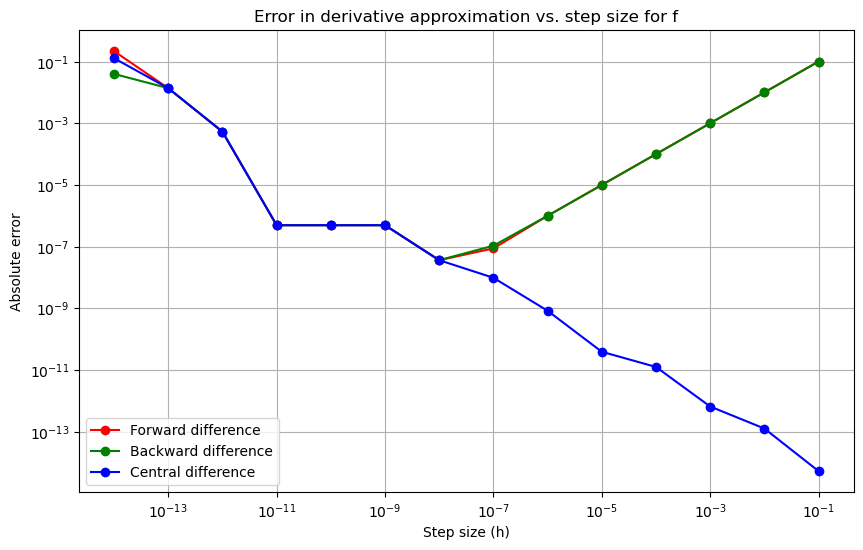
This plot will show how the error decreases as we make \( h \) smaller, confirming our understanding of derivatives through practical implementation.

It's a dragon!

Observations

• The plot shows error vs. step size.
• As we reduce \( h \), the error decreases initially, which is expected.
• Around \( 10^{-8} \), there's an inflection point where the error starts to increase.
• This indicates that beyond a certain small \( h \), our numerical method for differentiation might not be optimal due to precision issues in floating-point arithmetic.

Our basic approach to estimate numerical derivatives works well until we hit very small step sizes where computational errors become significant.

Three Methods to Numerically Estimate Derivatives

There are three common ways to approximate derivatives numerically. Let me explain each:

1. Forward Difference

\[ \frac{df}{dx} \approx \frac{f(x + h) - f(x)}{h} \]

• Why 'Forward'? Because we're looking at how the function changes when we move \( x \) in the positive direction by a small amount \( h \).

2. Backward Difference

\[ \frac{df}{dx} \approx \frac{f(x) - f(x - h)}{h} \]

• Why 'Backward'? This method measures the change in the function by moving \( x \) slightly in the negative direction.

3. Central Difference

\[ \frac{df}{dx} \approx \frac{f(x + h) - f(x - h)}{2h} \]

• The Process:
• We take the average of the forward and backward differences to get this formula.

• Simplification leads to dropping common terms and results in the formula above.

• Why 'Central'? This method balances both directions, often providing the most accurate approximation of the derivative.

The Central Difference is usually the most precise for estimating derivatives numerically due to its symmetry and error cancellation properties.

Comparing Three Numerical Differentiation Methods

Let's program and compare the performance of three numerical differentiation methods: Forward, Backward, and Central differences.

The Functions

We already have ndiff for forward difference. Let's implement backward and central differences:

def fdiff(f, x, h=1e-2):
    return (f(x + h) - f(x)) / h

def bdiff(f, x, h=1e-2):
    return (f(x) - f(x - h)) / h

def cdiff(f, x, h=1e-2):
    return (f(x + h) - f(x - h)) / (2 * h)

Testing with Functions

Exponential Function

\[ \frac{d}{dx}e^x = e^x \]

import numpy as np

def exp(x):
    return np.exp(x)

def d_exp(x):
    return np.exp(x)

x = 3
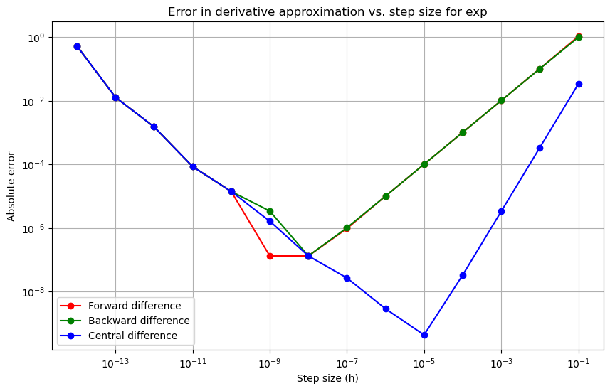
plot_errors(exp, d_exp, x)

Exponential Function

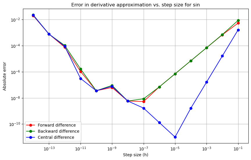
Sine Function

\[ \frac{d}{dx}sin(x) = cos(x) \]

def sin(x):
    return np.sin(x)

def d_sin(x):
    return np.cos(x)

x = 3
plot_errors(sin, d_sin, x)

Sin Function

Hyperbolic Tangent

\[ \frac{d}{dx}tanh(x) = 1 - tanh^2(x) \]

def tanh(x):
    return np.tanh(x)

def d_tanh(x):
    return 1 - np.tanh(x)**2

x = 3
plot_errors(tanh, d_tanh, x)

Hyperbolic Tangent Function

Observations

• Central Difference is generally more precise, particularly at smaller step sizes.
• Forward and Backward methods show similar error behavior, but Central difference often results in lower errors, especially for \( h \approx 10^{-5} \).
• The performance can vary slightly based on the function being differentiated, but Central difference consistently outperforms the others in accuracy.

Fun Fact:

The symmetric difference quotient, also known as the central difference, is used as the method for approximating derivatives in various calculators. Specifically, TI-82, TI-83, TI-84, and TI-85 calculators all implement this technique with a standard step size of \( h = 0.001 \).

Comments