Classification in Depth – Cross-Entropy & Softmax
Fashion-MNIST is a dataset created by Zalando Research as a drop-in replacement for MNIST. It consists of 70,000 grayscale images (28×28 pixels) categorized into 10 different classes of clothing, such as shirts, sneakers, and coats. Your mission? Train a model to classify these fashion items correctly!
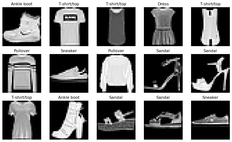
Fashion-MNIST Dataset Visualization
Check the jupyter notebook for this chapter
You can check my post Dive into Learning from Data - MNIST Video Adventure to understand the original MNIST challenge. Fashion-MNIST is a similar challenge - but this time, we're classifying clothing items instead of handwritten digits.
Unlike MNIST, where a simple Feed-Forward Neural Network might achieve near-perfect accuracy, Fashion-MNIST is a bit more challenging due to the complexity of clothing patterns. But that won't stop us from trying! Let's download the dataset and plot some sample images.
import matplotlib.pyplot as plt
from sklearn.datasets import fetch_openml

# Fetch the Fashion MNIST dataset from OpenML
fashion_mnist = fetch_openml('Fashion-MNIST', version=1, as_frame=False)

# Separate the features (images) and labels
X, y = fashion_mnist['data'], fashion_mnist['target']

# Convert labels to integers (since OpenML may return them as strings)
y = y.astype(int)


# Define label names for Fashion MNIST classes
label_names = [
    "T-shirt/top", "Trouser", "Pullover", "Dress", "Coat",
    "Sandal", "Shirt", "Sneaker", "Bag", "Ankle boot"
]

# Plot some sample images
fig, axes = plt.subplots(3, 5, figsize=(10, 6))
axes = axes.ravel()

for i in range(15):
    img = X[i].reshape(28, 28)  # Reshape the 1D array into a 28x28 image
    axes[i].imshow(img, cmap='gray')  # Display in grayscale
    axes[i].set_title(label_names[y[i]])  # Set label as title
    axes[i].axis('off')  # Hide axis

plt.tight_layout()
plt.show()
Output:
Fashion-MNIST Dataset Visualization
We need to prepare the data for training, so let's split the dataset into training and testing sets. This helps us train our model on one part of the data and test it on another. The main goal of training is to create a generalized solution that works on new, unseen data. To measure performance on unseen data, we set aside a portion of the dataset that won't be used during training. Instead, we use it after training to evaluate the model's accuracy.
# Train/test split
X_train, X_test, y_train, y_test = train_test_split(
    X, y, test_size=0.2, random_state=42
)

# Convert labels to integers
y_train, y_test = y_train.astype(int), y_test.astype(int)
Let's also convert the labels to one-hot format. One-hot labels are used because they make training more stable and efficient. They allow neural networks to treat each class independently, preventing unintended relationships between class indices. This is especially useful for classification tasks with softmax activation, ensuring proper probability distribution and better gradient flow.
# Convert labels to one-hot encoding
num_classes = 10
y_train_one_hot = np.eye(num_classes)[y_train]
y_test_one_hot = np.eye(num_classes)[y_test]
np.eye and one-hot encoding
We use np.eye(num_classes), which creates an identity matrix of size num_classes × num_classes.
Output:
Indexing withy_train = [2, 0, 3, 1] (np.eye(num_classes)[y_train])
Final One-Hot Encoded Output:
np.eye(num_classes) gives a lookup table where each row is a one-hot vector, indexing with y_train selects the correct rows for the given labels. It's a fast and memory-efficient way to convert class indices to one-hot encoding.
For data preprocessing let's use the MinMaxScaler. In short - MinMaxScaler scales features to a fixed range, usually [0, 1], improving model performance and stability.
from sklearn.preprocessing import MinMaxScaler

# Rescale
scaler = MinMaxScaler()
X_train = scaler.fit_transform(X_train)
X_test = scaler.transform(X_test)
You can check my post Dive into Learning from Data - MNIST Video Adventure, where we cracked the MNIST challenge and analyzed the image data.
CrossEntropyLoss and Softmax
In this problem, we have 10 different classes of clothing: ["T-shirt/top", "Trouser", "Pullover", "Dress", "Coat", "Sandal", "Shirt", "Sneaker", "Bag", "Ankle boot"]
Since we are dealing with multiple classes instead of just two, we need to scale up the entropy from BinaryEntropyLoss to CrossEntropyLoss. And the Sigmoid function is not the best choice for this task. Sigmoid outputs probabilities for each class independently, which is not good for multi-class classification. Instead, we need to assign probabilities across multiple classes, ensuring they sum to 1. A much better approach is to use the Softmax function, which converts raw model outputs (logits) into a probability distribution over all classes. This allows our model to make more accurate predictions by selecting the class with the highest probability.
In multiclass classification, the combination of Softmax + Cross-Entropy Loss has a unique property that simplifies the backward pass.
The Softmax function is defined as: \(S_i = \frac{e^{z_i}}{\sum_{j} e^{z_j}}\) and its derivative forms a Jacobian matrix:
This Jacobian matrix is \(N \times N\) (where \(N\) is the number of classes), which makes direct backpropagation inefficient.
But, the Cross-Entropy Loss \(L = -\sum_{i} y_i \log(S_i)\), and its gradient after softmax is simply:
The Softmax Jacobian cancels out with the Cross-Entropy derivative, so we avoid computing the full Jacobian. Instead, Softmax directly passes the gradient from Cross-Entropy, making backpropagation simpler and more efficient!
Why does the derivative of Cross-Entropy take the form \(\frac{\partial L}{\partial z_i} = S_i - y_i\)?
The Cross-Entropy Loss function is \(L = -\sum_{i} y_i \log(S_i)\), where \(y_i\) is the one-hot encoded true label (\(y_i = 1\) for the correct class, 0 otherwise). \(S_i\) is the softmax output (predicted probability for class \(i\)).
Now, let's compute the derivative of \(L\) with respect to \(S_i\):
However, the goal is to compute the gradient with respect to \(z_i\) (the input logits), not \(S_i\). This is where the Softmax derivative comes in. Softmax is defined as:
The derivative of \(S_i\) with respect to \(z_j\) gives a Jacobian matrix:
This means that if we want to find how the loss \(L\) changes with respect to \(z_i\), we need to apply the chain rule:
Substituting:
and
Let's expand:
Breaking it into cases:
- Diagonal term (\(i = j\)):
- Off-diagonal terms (\(i \neq j\)):
Summing over all \(j\), we get:
Since \(y\) is a one-hot vector, only one \(y_j = 1\), and all others are 0, meaning:
Intuition Behind Cancellation
Instead of explicitly computing the full Softmax Jacobian, the multiplication of the Cross-Entropy derivative and the Softmax Jacobian simplifies directly to \(S - y\).
- This happens because the off-diagonal terms in the Jacobian sum cancel out in the chain rule application.
- The result is a simple gradient computation without the need for the full Jacobian matrix.
This is why, in backpropagation, the Softmax layer doesn't need to explicitly compute its Jacobian. Instead, we can directly use:
to efficiently update the parameters in neural network training.
CrossEntropyLoss Implementation
class CrossEntropyLoss(Module):
    def forward(self, pred: np.ndarray, target: np.ndarray, epsilon: float = 1e-7) -> float:
        r"""
        Compute the Cross-Entropy loss for multiclass classification.

        Args:
            pred (np.ndarray): The predicted class probabilities from the model (output of softmax).
            target (np.ndarray): The one-hot encoded true target values.
            epsilon (float): A small value to avoid log(0) for numerical stability.

        Returns:
            float: The computed Cross-Entropy loss. Scalar for multiclass classification.
        """
        # Clip predictions to avoid log(0)
        pred = np.clip(pred, epsilon, 1. - epsilon)

        # Compute cross-entropy loss for each example
        loss = -np.sum(target * np.log(pred), axis=1)  # sum over classes for each example

        # Return the mean loss over the batch
        return np.mean(loss)

    def backward(self, pred: np.ndarray, target: np.ndarray, epsilon: float = 1e-7) -> np.ndarray:
        r"""
        Compute the gradient of the Cross-Entropy loss with respect to the predicted values.

        Args:
            pred (np.ndarray): The predicted class probabilities from the model (output of softmax).
            target (np.ndarray): The one-hot encoded true target values.
            epsilon (float): A small value to avoid division by zero for numerical stability.

        Returns:
            np.ndarray: The gradient of the loss with respect to the predictions.
        """

        # Clip predictions to avoid division by zero
        pred = np.clip(pred, epsilon, 1. - epsilon)

        # Compute the gradient of the loss with respect to predictions
        grad = pred - target  # gradient of cross-entropy w.r.t. predictions

        return grad
Now, let's see how this is efficiently handled in the backward pass of Softmax. The naive approach would be to compute the full Softmax Jacobian matrix, which has \(N \times N\) elements (where \(N\) is the number of classes). However, explicitly storing and multiplying by this matrix is computationally expensive. Instead, we take a more efficient approach using vectorized computation.
In the backward pass, we receive \(d_{\text{out}} = S - y\), which is the gradient of Cross-Entropy Loss with respect to Softmax outputs. The goal is to compute \(\frac{\partial L}{\partial z}\), the gradient of the loss with respect to logits.
The key observation is that for each example in the batch, the gradient of Softmax with respect to logits can be expressed as:
Summing over all \(j\), we get:
where \(d_{\text{out}} = S - y\) is the gradient from Cross-Entropy and the term \(\sum_j d_{\text{out}_j} S_j\) efficiently accounts for the interaction between all class probabilities.
Finally the Softmax.backward() function:
def backward(self, d_out: np.ndarray) -> np.ndarray:
    return self.output * (d_out - np.sum(d_out * self.output, axis=1, keepdims=True))
Instead of explicitly constructing the Jacobian, we directly compute the Jacobian-vector product, which is all we need for backpropagation. This avoids unnecessary computations, making the Softmax backward pass efficient and numerically stable.
Softmax Implementation
class Softmax(Module):
    """Softmax function and its derivative for backpropagation."""

    def forward(self, x: np.ndarray) -> np.ndarray:
        """
        Compute the Softmax of the input.
        Args:
            x (np.ndarray): Input array of shape (batch_size, n_classes).
        Returns:
            np.ndarray: Softmax probabilities.
        """

        # Subtract max for numerical stability
        exp_x = np.exp(x - np.max(x, axis=1, keepdims=True))
        self.output = exp_x / np.sum(exp_x, axis=1, keepdims=True)
        return self.output

    def backward(self, d_out: np.ndarray) -> np.ndarray:
        """
        Compute the gradient of the loss with respect to the input of the softmax.
        Args:
            d_out (np.ndarray): Gradient of the loss with respect to the softmax output.
                                Shape: (batch_size, n_classes).
        Returns:
            np.ndarray: Gradient of the loss with respect to the input of the softmax.
                        Shape: (batch_size, n_classes).
        """

        # Compute batch-wise Jacobian-vector product without explicit Jacobian computation
        return self.output * (d_out - np.sum(d_out * self.output, axis=1, keepdims=True))
The combination of Softmax + Cross-Entropy Loss simplifies backpropagation significantly. Instead of computing the full Jacobian, the Softmax layer directly propagates the gradient. This is why deep learning frameworks implement Softmax and Cross-Entropy together, optimizing for both performance and numerical stability!
SGD vs Fashion-MNIST
Let's prepare the model, loss function and use the SGD optimizer.
input_dims = 784

model = Sequential([
    Linear(input_dims, 784, init_method="he_leaky"),
    LeakyReLU(alpha=0.01),
    Linear(784, 256, init_method="he_leaky"),
    LeakyReLU(alpha=0.01),
    Linear(256, 128, init_method="he_leaky"),
    LeakyReLU(alpha=0.01),
    Linear(128, 10, init_method="xavier"),  # 10 output logits for Fashion-MNIST
    Softmax()
])

bce = CrossEntropyLoss()
optimizer = SGD(lr=0.01, momentum=0.9)
Now, let's build and run our training loop for Fashion-MNIST:
from sklearn.metrics import accuracy_score


# Hyperparameters
epochs = 20
batch_size = 128


# Training loop
for epoch in range(epochs):
    # Shuffle training data - can help prevent overfitting!
    # Stochastic batch of data for the training process!
    indices = np.random.permutation(X_train.shape[0])
    X_train_shuffled, y_train_shuffled = X_train[indices], y_train_one_hot[indices]

    total_loss = 0
    num_batches = X_train.shape[0] // batch_size

    for i in range(0, X_train.shape[0], batch_size):
        # Use a stochastic batch of data for training
        X_batch = X_train_shuffled[i:i+batch_size]
        y_batch = y_train_shuffled[i:i+batch_size]

        #############
        # Core steps!
        #############

        # Forward pass
        preds = model(X_batch)
        loss = bce(preds, y_batch)

        # Zero grad before the backward pass!
        model.zero_grad()

        # Backward pass
        d_loss = bce.backward(preds, y_batch)
        model.backward(d_loss)

        # Update weights
        optimizer.step(model)

        total_loss += loss

    # Compute average loss
    avg_loss = total_loss / num_batches
    print(f"Epoch {epoch+1}/{epochs}, Loss: {avg_loss:.4f}")


# Evaluation
y_pred = model(X_test)
y_pred_labels = np.argmax(y_pred, axis=1)
accuracy = accuracy_score(y_test, y_pred_labels)

print(f"Test Accuracy: {accuracy * 100:.2f}%")
I shuffled the training data, which can help prevent overfitting because the training algorithm might make sense of the sequence of batches and start to adjust the weights in the direction of the training batches. Remember, we use a stochastic batch of data for the training process and compute the gradient direction of this mini-batch of data.
Output:
Epoch 1/20, Loss: 0.5885
Epoch 2/20, Loss: 0.4156
Epoch 3/20, Loss: 0.3807
Epoch 4/20, Loss: 0.3570
Epoch 5/20, Loss: 0.3370
Epoch 6/20, Loss: 0.3236
Epoch 7/20, Loss: 0.3089
Epoch 8/20, Loss: 0.3052
Epoch 9/20, Loss: 0.2970
Epoch 10/20, Loss: 0.2837
Epoch 11/20, Loss: 0.2757
Epoch 12/20, Loss: 0.2712
Epoch 13/20, Loss: 0.2636
Epoch 14/20, Loss: 0.2608
Epoch 15/20, Loss: 0.2513
Epoch 16/20, Loss: 0.2448
Epoch 17/20, Loss: 0.2438
Epoch 18/20, Loss: 0.2357
Epoch 19/20, Loss: 0.2325
Epoch 20/20, Loss: 0.2311
Test Accuracy: 89.94%
Also we can check the extended metrics:
import pandas as pd
from sklearn.metrics import precision_score, recall_score, f1_score

# Calculate precision, recall, and F1 scores per class
precision_per_class = precision_score(y_test, y_pred_labels, average=None)
recall_per_class = recall_score(y_test, y_pred_labels, average=None)
f1_per_class = f1_score(y_test, y_pred_labels, average=None)

# Create a DataFrame to store the metrics per class
metrics_df = pd.DataFrame({
    'Class': range(len(precision_per_class)),
    'Precision': precision_per_class,
    'Recall': recall_per_class,
    'F1-Score': f1_per_class
})

# Display the table
print(metrics_df)
Output:
   Class  Precision    Recall  F1-Score
0      0   0.830812  0.866571  0.848315
1      1   0.991254  0.970043  0.980534
2      2   0.870843  0.800284  0.834074
3      3   0.877632  0.920635  0.898619
4      4   0.791472  0.875461  0.831351
5      5   0.973629  0.968254  0.970934
6      6   0.759445  0.700071  0.728550
7      7   0.939844  0.977189  0.958153
8      8   0.984733  0.961252  0.972851
9      9   0.978556  0.954672  0.966467
Not bad for SGD! We can use SGD with momentum and gradient clipping as an optimization baseline. From here, we can aim to surpass this baseline by exploring more advanced optimization techniques!